Functional Auto Encoder with R Keras

tidymodels

tensorflow

code

Author

Bruno Testaguzza Carlin

Published

March 31, 2023

Objective

This is a somewhat simple post trying to mimic the guides on auto encoders present in Third example: Anomaly detection

Libraries

Do keep in mind that in order to use tensorflow you should run

tensorflow::install_tensorflow()

Code

library(keras3)
library(rsample) |> suppressMessages()
library(recipes) |> suppressMessages()
library(ggplot2)
library(tidyr)

Code

reticulate::use_virtualenv('py399')

Download The Dataset

Code

dataframe <-  readr::read_csv('http://storage.googleapis.com/download.tensorflow.org/data/ecg.csv',col_names = FALSE)

Rows: 4998 Columns: 141
── Column specification ────────────────────────────────────────────────────────
Delimiter: ","
dbl (141): X1, X2, X3, X4, X5, X6, X7, X8, X9, X10, X11, X12, X13, X14, X15,...

ℹ Use `spec()` to retrieve the full column specification for this data.
ℹ Specify the column types or set `show_col_types = FALSE` to quiet this message.

Code

dataframe |> head()

Code

raw_data <- dataframe

Preprocessing

Split the data

Code

set.seed(20)

raw_data_split <- initial_split(raw_data,prop = .8)

train_data <- training(raw_data_split)

test_data <- testing(raw_data_split)

Normalize the data to [0,1].

Code

target_varible <- raw_data[,ncol(raw_data)] |> names()

recipe_data <- recipe(train_data) |> 
  update_role(target_varible,new_role = 'outcome') |> 
  update_role(-target_varible,new_role = 'predictor') |> 
  step_range(all_predictors(),min = 0,max = 1)

Warning: Using an external vector in selections was deprecated in tidyselect 1.1.0.
ℹ Please use `all_of()` or `any_of()` instead.
  # Was:
  data %>% select(target_varible)

  # Now:
  data %>% select(all_of(target_varible))

See <https://tidyselect.r-lib.org/reference/faq-external-vector.html>.

Code

preped_recipe_data <- recipe_data |> prep(train_data)

baked_train_data <- preped_recipe_data |> bake(new_data = NULL)
baked_test_data <- preped_recipe_data |> bake(test_data)

Separate datasets for future usage

You will train the autoencoder using only the normal rhythms

Which are labeled in this dataset as 1.

Separate the normal rhythms from the abnormal rhythms.

Code

normal_train_data <-  baked_train_data |> filter(get(target_varible) == 1)
normal_test_data <-  baked_test_data |> filter(get(target_varible) == 1)

anomalous_train_data <-  baked_train_data |> filter(get(target_varible) == 0)
anomalous_test_data <-  baked_test_data |> filter(get(target_varible) == 0)

See the data

Normal ECG

Code

# Plot a normal ECG.

normal_train_data |> 
  head(1) |>
  pivot_longer(-target_varible) |>
  mutate(name = name |> stringr::str_extract('\\d+') |> as.numeric()) |> 
  ggplot(aes(x = name,y = value)) +
  geom_line() +
  theme_minimal() +
  labs(title = 'A Normal ECG',x = NULL,y = NULL)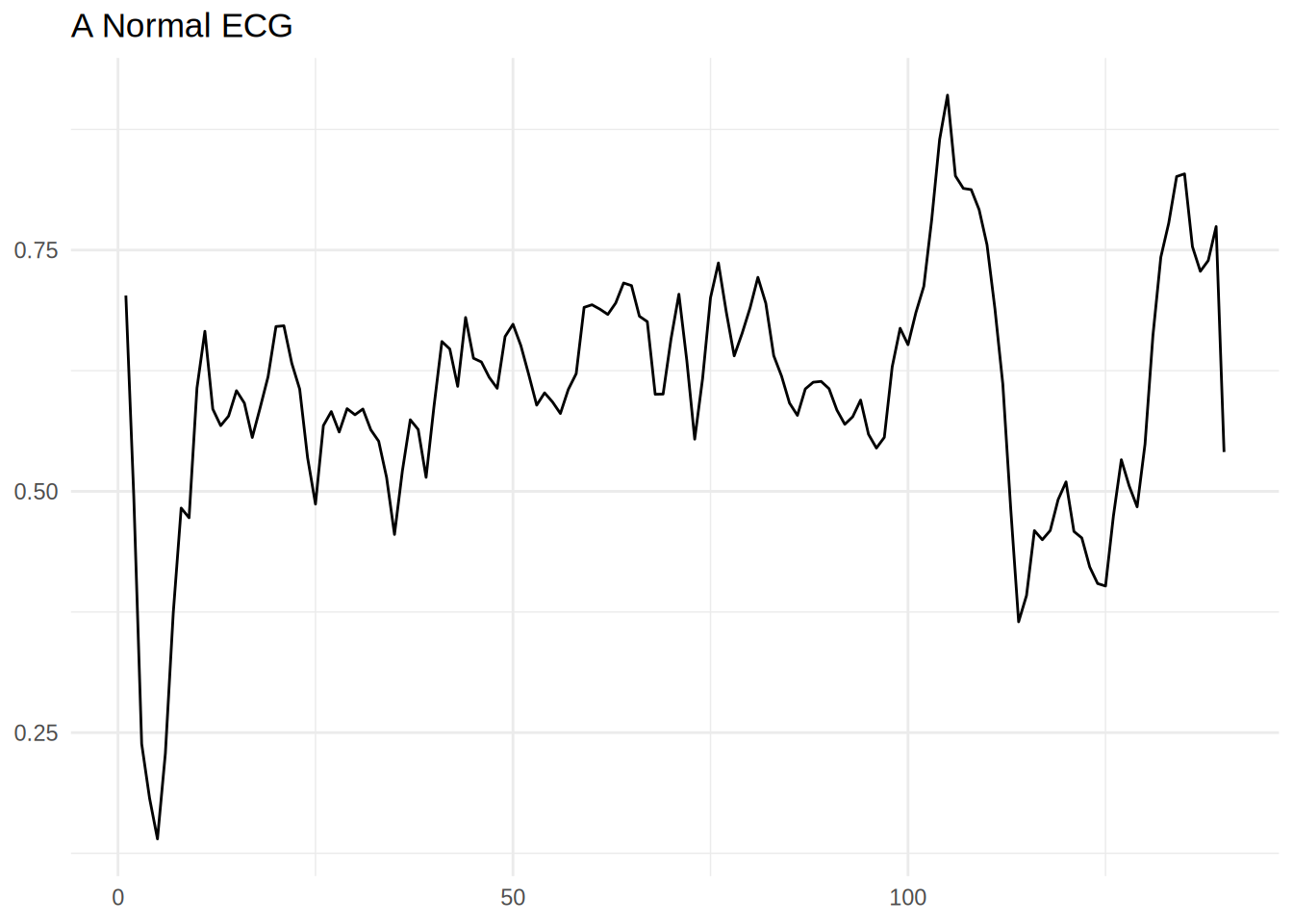

Anomalous ECG

Code

anomalous_train_data |> 
  head(1) |>
  pivot_longer(-target_varible) |>
  mutate(name = name |> stringr::str_extract('\\d+') |> as.numeric()) |> 
  ggplot(aes(x = name,y = value)) +
  geom_line() +
  theme_minimal() +
  labs(title = 'A Anomalous ECG',x = NULL,y = NULL)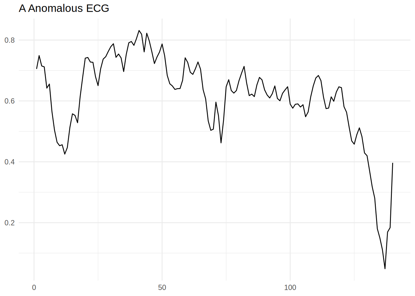

Create Matrixes for tensorflow

Code

normal_train_data_x <- normal_train_data |>
  select(-target_varible) |> 
  as.matrix()

normal_test_data_x <- normal_test_data |>
  select(-target_varible) |> 
  as.matrix()

test_data_x <- baked_test_data |> 
  select(-target_varible) |> 
  as.matrix()

anomalous_test_data_x <- anomalous_test_data |> 
  select(-target_varible) |> 
  as.matrix()

Build The Auto Encoder- Using the functional api

Discover the input and output dimensions

Code

# dim_features is the dimension of your features
dim_features <- normal_train_data |> select(-target_varible) |> ncol()

# latent dim is usually the smallest layer of the network at the end of the encoder model
latent_dim <- 8

Define the encoder

Code

import sys
sys.executable

'/home/carlin/.virtualenvs/py399/bin/python'

Code

#|warning: false
encoder_input <- layer_input(shape = c(dim_features), name = "features")

encoder_output <- encoder_input |> 
  layer_dense(32,activation = "relu") |> 
  layer_dense(16,activation = "relu") |>
  layer_dense(latent_dim,activation = "relu")

encoder <- keras_model(encoder_input, encoder_output, name = "encoder")
encoder

Model: "encoder"
┏━━━━━━━━━━━━━━━━━━━━━━━━━━━━━━━━━━━┳━━━━━━━━━━━━━━━━━━━━━━━━━━┳━━━━━━━━━━━━━━━┓
┃ Layer (type)                      ┃ Output Shape             ┃       Param # ┃
┡━━━━━━━━━━━━━━━━━━━━━━━━━━━━━━━━━━━╇━━━━━━━━━━━━━━━━━━━━━━━━━━╇━━━━━━━━━━━━━━━┩
│ features (InputLayer)             │ (None, 140)              │             0 │
├───────────────────────────────────┼──────────────────────────┼───────────────┤
│ dense (Dense)                     │ (None, 32)               │         4,512 │
├───────────────────────────────────┼──────────────────────────┼───────────────┤
│ dense_1 (Dense)                   │ (None, 16)               │           528 │
├───────────────────────────────────┼──────────────────────────┼───────────────┤
│ dense_2 (Dense)                   │ (None, 8)                │           136 │
└───────────────────────────────────┴──────────────────────────┴───────────────┘
 Total params: 5,176 (20.22 KB)
 Trainable params: 5,176 (20.22 KB)
 Non-trainable params: 0 (0.00 B)

Define Decoder

Code

decoder_input <- layer_input(shape = c(latent_dim), name = "latent_dim")

decoder_output <- decoder_input |> 
  layer_dense(16,activation = "relu") |> 
  layer_dense(32,activation = "relu") |>
  layer_dense(dim_features,activation = "sigmoid")

decoder <- keras_model(decoder_input, decoder_output, name = "decoder")
decoder

Model: "decoder"
┏━━━━━━━━━━━━━━━━━━━━━━━━━━━━━━━━━━━┳━━━━━━━━━━━━━━━━━━━━━━━━━━┳━━━━━━━━━━━━━━━┓
┃ Layer (type)                      ┃ Output Shape             ┃       Param # ┃
┡━━━━━━━━━━━━━━━━━━━━━━━━━━━━━━━━━━━╇━━━━━━━━━━━━━━━━━━━━━━━━━━╇━━━━━━━━━━━━━━━┩
│ latent_dim (InputLayer)           │ (None, 8)                │             0 │
├───────────────────────────────────┼──────────────────────────┼───────────────┤
│ dense_3 (Dense)                   │ (None, 16)               │           144 │
├───────────────────────────────────┼──────────────────────────┼───────────────┤
│ dense_4 (Dense)                   │ (None, 32)               │           544 │
├───────────────────────────────────┼──────────────────────────┼───────────────┤
│ dense_5 (Dense)                   │ (None, 140)              │         4,620 │
└───────────────────────────────────┴──────────────────────────┴───────────────┘
 Total params: 5,308 (20.73 KB)
 Trainable params: 5,308 (20.73 KB)
 Non-trainable params: 0 (0.00 B)

Define The Auto Encoder

Code

encoded <- encoder(encoder_input)
decoded <- decoder(encoded)
autoencoder <- keras_model(encoder_input, decoded,
                           name = "autoencoder")
autoencoder

Model: "autoencoder"
┏━━━━━━━━━━━━━━━━━━━━━━━━━━━━━━━━━━━┳━━━━━━━━━━━━━━━━━━━━━━━━━━┳━━━━━━━━━━━━━━━┓
┃ Layer (type)                      ┃ Output Shape             ┃       Param # ┃
┡━━━━━━━━━━━━━━━━━━━━━━━━━━━━━━━━━━━╇━━━━━━━━━━━━━━━━━━━━━━━━━━╇━━━━━━━━━━━━━━━┩
│ features (InputLayer)             │ (None, 140)              │             0 │
├───────────────────────────────────┼──────────────────────────┼───────────────┤
│ encoder (Functional)              │ (None, 8)                │         5,176 │
├───────────────────────────────────┼──────────────────────────┼───────────────┤
│ decoder (Functional)              │ (None, 140)              │         5,308 │
└───────────────────────────────────┴──────────────────────────┴───────────────┘
 Total params: 10,484 (40.95 KB)
 Trainable params: 10,484 (40.95 KB)
 Non-trainable params: 0 (0.00 B)

Fit the model

Code

history <- autoencoder |>
  compile(loss = "mae",
          optimizer = "adam") |>
  fit(
    x = normal_train_data_x,
    y = normal_train_data_x,
    epochs = 20,
    batch_size = 512,
    validation_data = list(
      test_data_x,
      test_data_x
    ),
    shuffle = TRUE
  )

Epoch 1/20
5/5 - 1s - 187ms/step - loss: 0.1349 - val_loss: 0.1405
Epoch 2/20
5/5 - 0s - 8ms/step - loss: 0.1308 - val_loss: 0.1346
Epoch 3/20
5/5 - 0s - 8ms/step - loss: 0.1234 - val_loss: 0.1252
Epoch 4/20
5/5 - 0s - 8ms/step - loss: 0.1132 - val_loss: 0.1158
Epoch 5/20
5/5 - 0s - 8ms/step - loss: 0.1036 - val_loss: 0.1086
Epoch 6/20
5/5 - 0s - 8ms/step - loss: 0.0942 - val_loss: 0.1005
Epoch 7/20
5/5 - 0s - 8ms/step - loss: 0.0844 - val_loss: 0.0936
Epoch 8/20
5/5 - 0s - 8ms/step - loss: 0.0759 - val_loss: 0.0877
Epoch 9/20
5/5 - 0s - 8ms/step - loss: 0.0686 - val_loss: 0.0833
Epoch 10/20
5/5 - 0s - 8ms/step - loss: 0.0627 - val_loss: 0.0799
Epoch 11/20
5/5 - 0s - 7ms/step - loss: 0.0582 - val_loss: 0.0778
Epoch 12/20
5/5 - 0s - 8ms/step - loss: 0.0551 - val_loss: 0.0765
Epoch 13/20
5/5 - 0s - 8ms/step - loss: 0.0531 - val_loss: 0.0757
Epoch 14/20
5/5 - 0s - 8ms/step - loss: 0.0516 - val_loss: 0.0752
Epoch 15/20
5/5 - 0s - 8ms/step - loss: 0.0503 - val_loss: 0.0746
Epoch 16/20
5/5 - 0s - 8ms/step - loss: 0.0494 - val_loss: 0.0745
Epoch 17/20
5/5 - 0s - 8ms/step - loss: 0.0486 - val_loss: 0.0742
Epoch 18/20
5/5 - 0s - 8ms/step - loss: 0.0480 - val_loss: 0.0741
Epoch 19/20
5/5 - 0s - 7ms/step - loss: 0.0475 - val_loss: 0.0740
Epoch 20/20
5/5 - 0s - 7ms/step - loss: 0.0471 - val_loss: 0.0739

Code

plot(history)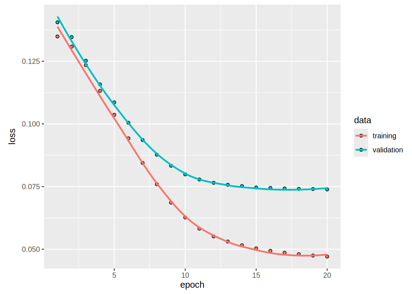

Plot the predictions

Reconstruction on Normal data

Code

encoded_data <- encoder |>
  predict(normal_test_data_x)

19/19 - 0s - 3ms/step

Code

decoded_data <- decoder |> 
  predict(encoded_data)

19/19 - 0s - 3ms/step

Code

decoded_data_to_plot <- decoded_data |> 
  head(1) |>
  as_tibble() |> 
  pivot_longer(everything(),values_to = 'Reconstruction') |> 
  mutate(name = name |> stringr::str_extract('\\d+') |> as.numeric())

Warning: The `x` argument of `as_tibble.matrix()` must have unique column names if
`.name_repair` is omitted as of tibble 2.0.0.
ℹ Using compatibility `.name_repair`.

Code

normal_test_data_to_plot <- normal_test_data_x |>
  head(1) |>
  as_tibble() |> 
  pivot_longer(everything(),values_to = 'Input')|> 
  mutate(name = name |> stringr::str_extract('\\d+')|> as.numeric())

data_to_plot <- decoded_data_to_plot |> 
  left_join(normal_test_data_to_plot,by = 'name')


data_to_plot |>
  pivot_longer(cols = -name,names_to = 'source') |> 
  ggplot(aes(x = name,y = value,colour = source,group = source)) + 
  geom_line() +
  theme_minimal() +
  labs(title = 'Recontruction on test data',x = NULL,y=NULL)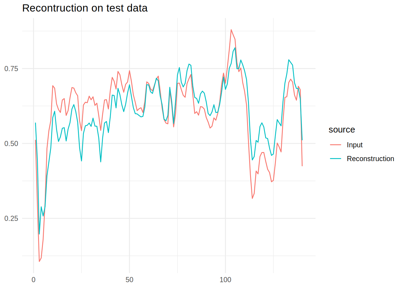

Reconstruction on Anomalous data

It is clear that the reconstruction can’t quite create the output, this is what we will exploit to define outliers.

Code

encoded_data <- encoder |>
  predict(anomalous_test_data_x)

14/14 - 0s - 2ms/step

Code

decoded_data <- decoder |> 
  predict(encoded_data)

14/14 - 0s - 1ms/step

Code

decoded_data_to_plot <- decoded_data |> 
  head(1) |>
  as_tibble() |> 
  pivot_longer(everything(),values_to = 'Reconstruction') |> 
  mutate(name = name |> stringr::str_extract('\\d+') |> as.numeric())

normal_test_data_to_plot <- anomalous_test_data_x |>
  head(1) |>
  as_tibble() |> 
  pivot_longer(everything(),values_to = 'Input')|> 
  mutate(name = name |> stringr::str_extract('\\d+')|> as.numeric())

data_to_plot <- decoded_data_to_plot |> 
  left_join(normal_test_data_to_plot,by = 'name')


data_to_plot |>
  pivot_longer(cols = -name,names_to = 'source') |> 
  ggplot(aes(x = name,y = value,colour = source,group = source)) + 
  geom_line() +
  theme_minimal() +
  labs(title = 'Recontruction on Anomalous test data',x = NULL,y=NULL)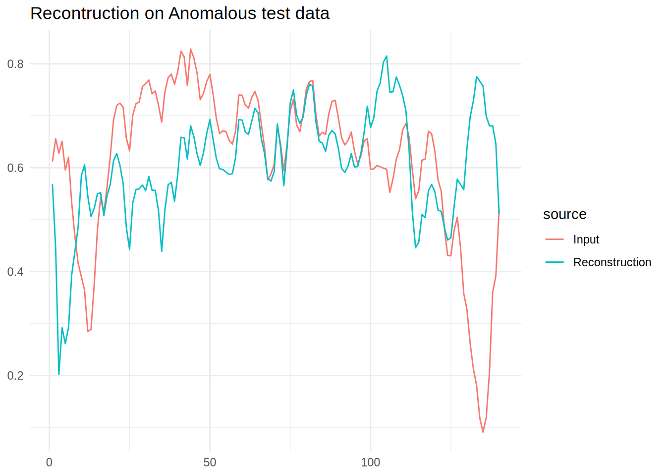

Detect anomalies

Discover the threshold to flag annomalies

Code

reconstructions <-  autoencoder |> predict(normal_train_data_x) |> as_tibble()

73/73 - 0s - 1ms/step

Code

train_data_tibble <- normal_train_data_x |> as_tibble()


train_loss = loss_mean_squared_error(as.matrix(reconstructions), as.matrix(train_data_tibble))

data_loss <- train_loss |> as.numeric() |> as_tibble()

data_loss |> 
  ggplot(aes(x = value)) +
  geom_histogram(bins = 50) +
  labs(title = 'Loss Normal Train Data',x = 'Train Loss', y = 'No of examples') +
  theme_minimal()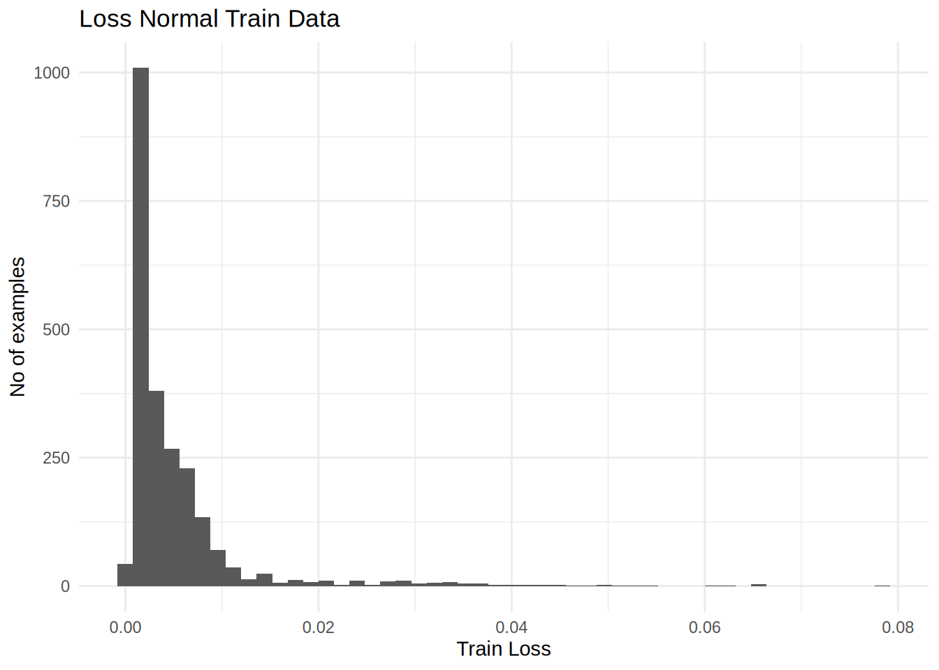

Code

threshold <-mean(train_loss) + sd(train_loss)

print(threshold |> as.numeric())

[1] 0.01256173

Completness

There are other strategies you could use to select a threshold value above which test examples should be classified as anomalous, the correct approach will depend on your dataset. You can learn more with the links at the end of this tutorial.

Strategy

Note

If you examine the reconstruction error for the anomalous examples in the test set, you’ll notice most have greater reconstruction error than the threshold. By varing the threshold, you can adjust the precision and recall of your classifier.

tidy.outliers

If you need something faster, and usually more practical do check out my package tidy.outliers for easy to use outlier detection methods.

Code

reconstructions <-  autoencoder |> predict(anomalous_test_data_x) |> as_tibble()

14/14 - 0s - 4ms/step

Code

anomalous_test_data_x_tibble <- anomalous_test_data_x |> as_tibble()

test_loss = loss_mean_squared_error(as.matrix(reconstructions), as.matrix(anomalous_test_data_x_tibble))

data_loss <- test_loss |> as.numeric() |> as_tibble()

data_loss |> 
  ggplot(aes(x = value)) +
  geom_histogram(bins = 50) +
  labs(title = 'Loss Anomalous Test Data',x = 'Test Loss', y = 'No of examples') +
  theme_minimal()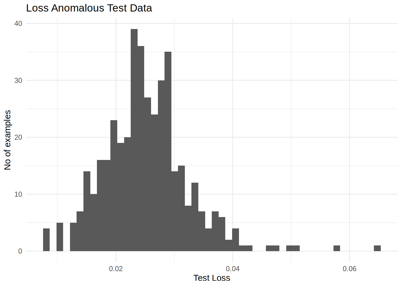

Classify anomalies

Code

predict_outlier <- function(model,data,threshold){
  reconstructions <-  model |> predict(data)
  loss <-  loss_mean_squared_error(reconstructions, data)
  df_result <- keras::k_less(loss,threshold) |>
    as.numeric() |> 
    as.factor() |> 
    as_tibble() |> 
    rename(estimate = value)
  return(df_result)
}

preds <- predict_outlier(autoencoder,anomalous_test_data_x,threshold)

14/14 - 0s - 2ms/step

Registered S3 methods overwritten by 'keras':
  method                               from  
  as.data.frame.keras_training_history keras3
  plot.keras_training_history          keras3
  print.keras_training_history         keras3
  r_to_py.R6ClassGenerator             keras3

Code

test_data <- anomalous_test_data |>
  select(target_varible) |> 
  rename(truth = target_varible) |> 
  mutate(truth = truth |> factor(levels = c(0,1)))

df_result <- test_data |> 
  bind_cols(preds)

df_result |> 
  yardstick::accuracy(truth = truth,estimate = estimate)

Code

df_result |> 
  yardstick::precision(truth = truth,estimate = estimate)

Code

df_result |> 
  yardstick::recall(truth = truth,estimate = estimate)

Changelog

2024-02-09 Updated to Keras3.

Next Steps

Check out the Tensorflow Next Steps